Classifying Handwritten Digits with Machine Learning

Overview

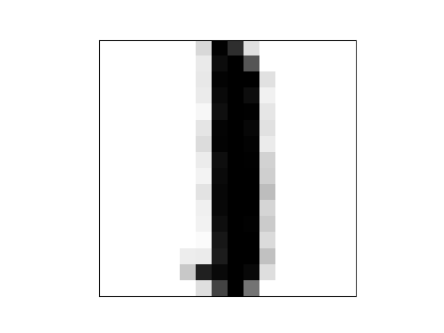
Digit 1

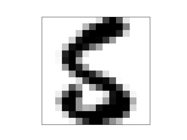
Digit 5

This project explores the classification of handwritten digits (1s vs 5s) using several machine learning techniques, focusing on feature engineering and algorithmic performance. The dataset consisted of grayscale digit images, and the primary objective was to separate the two classes reliably by extracting informative features and applying linear and logistic approaches.

When working with handwritten digits, it's important to recognize that no two digits will look exactly the same - and some people frankly have terrible handwriting. This inherent variability means achieving zero error is essentially impossible. The best we can do is build a model that makes the most educated guess possible based on the patterns it learns from the training data.

Feature Engineering

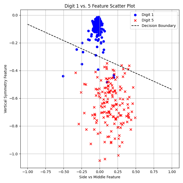
I chose and implemented two custom features to enable separation of the digits:

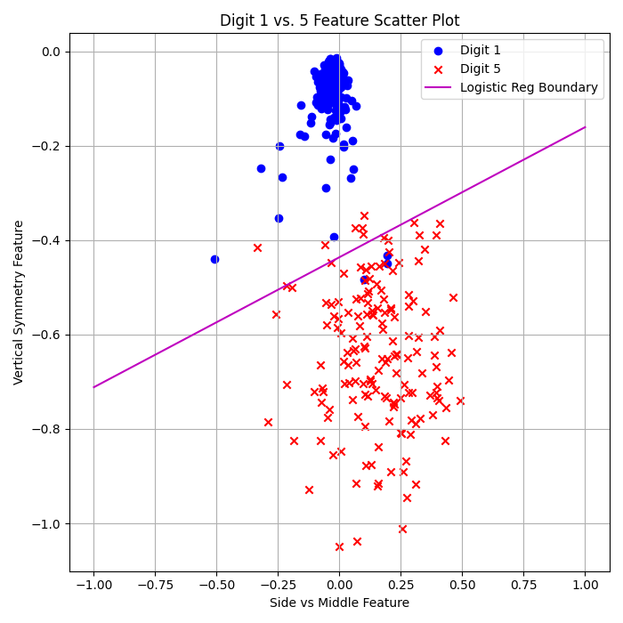
• Vertical Symmetry: Measures the absolute difference between intensities of the left and right halves of each image. More negative values indicate less symmetry.
• Side vs Middle Intensity: Compares the summed pixel intensity of the outer columns (left/right) to the central columns (middle) of the image. Returns a proportion that highlights where the digit ink is most concentrated.

def vertical_symmetry_feature(image):
    left_half = image[:, :8]
    right_half = np.fliplr(image[:, 8:])
    symmetry = -np.sum(np.abs(left_half - right_half)) / (16*8)
    return float(symmetry)

def side_vs_middle_feature(image):
    left = np.sum(image[:, 0:5])
    middle = np.sum(image[:, 5:11])
    right = np.sum(image[:, 11:16])
    sides = left + right
    prop_sides = sides / (2*16*5)
    prop_middle = middle / (16*6)
    return float(prop_sides - prop_middle)
                        

Classification Algorithms

After feature extraction, three main algorithms were tested:

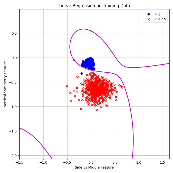
• Linear Regression + Pocket PLA: Used regression weights as initialization for the perceptron-like pocket algorithm, improving robustness.
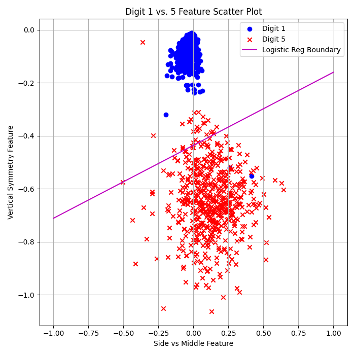
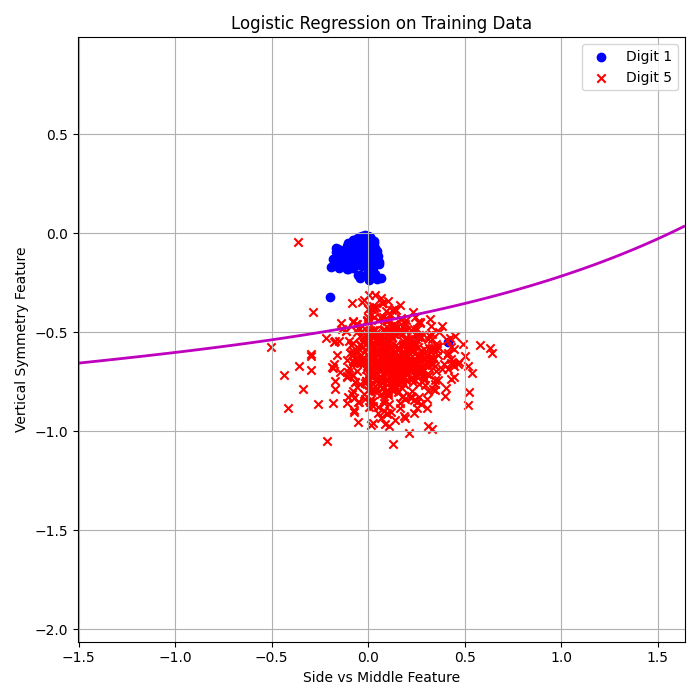
• Logistic Regression (Batch Gradient Descent): Traditional logistic regression using all data to update weights in each step.
• Logistic Regression (Stochastic Gradient Descent): Faster convergence by updating on random individual samples; surprisingly, gave the best results in this scenario.

def lin_reg(X, y):
    X_bias = np.hstack([np.ones((X.shape[0], 1)), X])
    w = np.linalg.pinv(X_bias.T @ X_bias) @ X_bias.T @ y
    return w

def pocket_pla(X, y, w_init, max_iter=1000):
    X_aug = np.hstack([np.ones((X.shape[0], 1)), X])
    w = w_init.copy()
    pocket_w = w.copy()
    best_error = np.sum(np.sign(X_aug @ w) != y)
    for iter_count in range(max_iter):
        predictions = np.sign(X_aug @ w)
        misclassified = np.where(predictions != y)[0]
        if len(misclassified) == 0:
            return pocket_w, iter_count
        i = misclassified[0]
        w = w + y[i] * X_aug[i]
        error = np.sum(np.sign(X_aug @ w) != y)
        if error < best_error:
            pocket_w = w.copy()
            best_error = error
    return pocket_w, best_error / y.shape[0]
                        

def log_reg(X, y):
    X_bias = np.hstack([np.ones((X.shape[0], 1)), X])
    w = np.zeros(X_bias.shape[1])
    lr = 0.01
    y_01 = (y + 1) // 2
    for iteration in range(5000):
        z = X_bias @ w
        probs = 1 / (1 + np.exp(-z))
        grad = (1/X_bias.shape[0]) * (X_bias.T @ (probs - y_01))
        w -= lr * grad
    return w

def stochastic_log_reg(X, y):
    X_bias = np.hstack([np.ones((X.shape[0], 1)), X])
    w = np.zeros(X_bias.shape[1])
    lr = 0.01
    y_01 = (y + 1) // 2
    for epoch in range(500):
        indices = np.random.permutation(X_bias.shape[0])
        for i in indices:
            z = X_bias[i] @ w
            prob = 1 / (1 + np.exp(-z))
            grad = (prob - y_01[i]) * X_bias[i]
            w -= lr * grad
    return w
                        

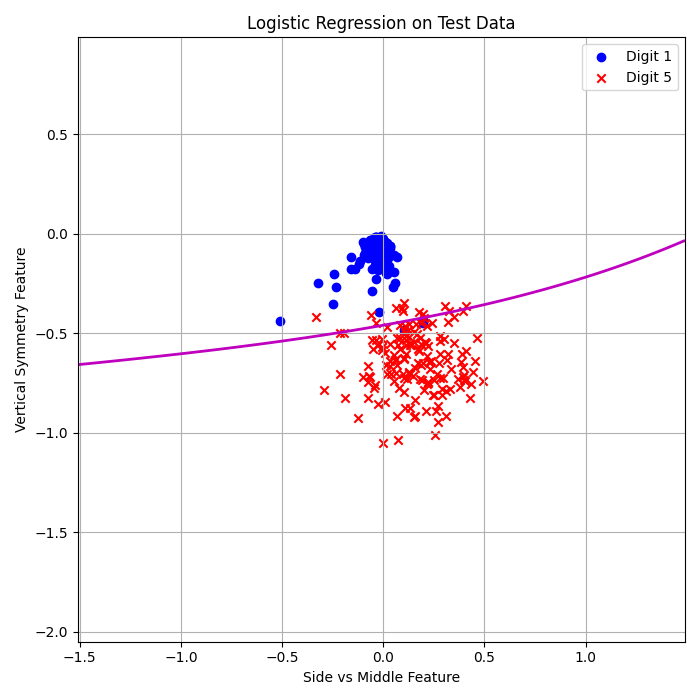
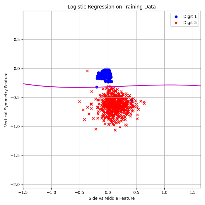
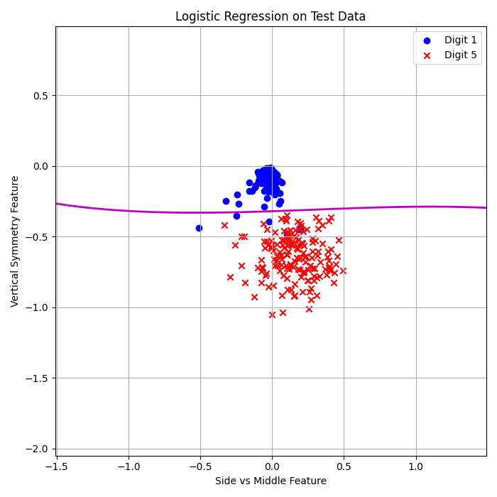
Results: Linear vs Logistic Regression

Each algorithm was run on both training and test sets, reporting both in-sample and out-of-sample errors. Stochastic logistic regression consistently achieved the lowest test errors.

Linear Regression (Training Data)

Linear Regression (Test Data)

Logistic Regression (Batch GD, Training)

Logistic Regression (Batch GD, Test)

Logistic Regression (Stochastic GD, Training)

Logistic Regression (Stochastic GD, Test)

I was actually shocked by how well this algorithm performed. Running 500 cycles gave the best outcome—even more iterations (1000, 2000, or 5000) degraded performance.

Bounded Error Interpretation

Using a conservative error bound of 0.05, we can establish confidence intervals for out-of-sample performance:

\( E_{\text{out}} \leq E_{\text{in}} + \delta \)
\( E_{\text{out}} \leq E_{\text{test}} + \delta \)

For Stochastic GD:
With \( E_{\text{in}} = 0.0019 \), \( \delta = 0.05 \): \( E_{\text{out}} \leq 0.0519 \)
With \( E_{\text{test}} = 0.0142 \), \( \delta = 0.05 \): \( E_{\text{out}} \leq 0.0642 \)

Third Order Polynomial Feature Expansion

I also experimented with third-order polynomial features to potentially improve classification boundaries - this is a more complicated model that could potentially better fit the data. However, when using more complex models, it is important to be careful about overfitting.

def poly3_features(f1, f2):
    return np.column_stack([
        np.ones_like(f1),      # bias
        f1, f2,
        f1**2, f1*f2, f2**2,
        f1**3, (f1**2)*f2, f1*(f2**2), f2**3
    ])

x1_min, x1_max = f1.min() - 1, f1.max() + 1
x2_min, x2_max = f2.min() - 1, f2.max() + 1
xx, yy = np.meshgrid(np.linspace(x1_min, x1_max, 200), np.linspace(x2_min, x2_max, 200))

# Flatten the grid to 1D arrays for feature expansion
xx_flat = xx.ravel()
yy_flat = yy.ravel()

# Compute polynomial features for all grid points
grid_poly = poly3_features(xx_flat, yy_flat)  # shape (N_grid, 10)
grid_poly =np.hstack([np.ones((grid_poly.shape[0], 1)), grid_poly])#bias to make both matrixes same size
Z = grid_poly @ w_final  # shape (N_grid,)
Z = Z.reshape(xx.shape)

#Linear Regression line for 3rd order
#plt.contour(xx, yy, Z, levels=[0], colors='m', linewidths=2)
                        

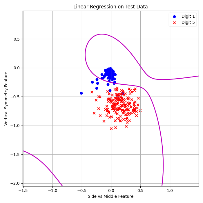
Linear + Pocket (3rd Order, Training)

Linear + Pocket (3rd Order, Test)

Logistic Regression (3rd Order, Training)

Logistic Regression (3rd Order, Test)

Stochastic Logistic Regression (3rd Order, Training)

Stochastic Logistic Regression (3rd Order, Test)

Conclusion

This project demonstrated the importance of using precise features and carefully selecting algorithms in machine learning. The stochastic gradient descent approach outperformed both linear and batch logistic regression overall, achieving remarkably low error rates. The third-order polynomial features showed mixed results—while they improved training performance in some cases, they also introduced slight overfitting in the Linear + Pocket model. This makes sense, as it's not like the third order polynomial is a cure-all - it's just another option for a model that could potentially better fit the data.

Overall, this was a really cool project that was my first real application of Machine Learning to a real problem. I learned a lot and look forward to applying these concepts to more complex problems in the future. If I were to consider expanding this project to distinguish between all digits, I would probably need to use a more complex model - more features, more complex algorithms, and I would probably separate it into several steps, with each step distinguishing between a different pair of digits.